
Want to put the math to the test? Drop a ball and feel the curve in action, try Plinko now at Plinko Ball Online.
If you’ve ever watched a chip bounce through pegs and wondered why the center pokies fill up, you’re already thinking about the plinko binomial distribution. In this guide, we break down the plinko math model and show how the plinko probability curve emerges from simple assumptions. We’ll cover the core binomial setup, derive the distribution, interpret the mean and variance, and show when real boards deviate from the ideal. We’ll also outline quick ways to compute or simulate odds so you can analyze any board design with confidence.
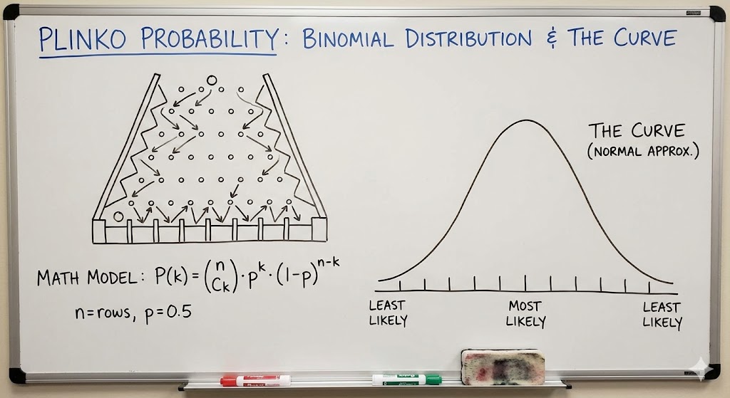
How Plinko Maps To A Binomial Process
Assumptions And Setup
To turn a Plinko board into math, we start with a few clean assumptions:
- The board has n rows of pegs. Each row forces the ball to choose left or right once.
- At each peg, the ball deflects independently of previous hits.
- The probability of going right on any given peg is p (and left is 1 − p). In the classic symmetric case, p = 0.5.
- The final landing slot is determined by how many times the ball goes right (or left) across those n decisions.
Under these assumptions, each drop is a sequence of n Bernoulli trials (right vs. left). That’s the exact binomial model that all reliable plinko strategy frameworks and most evidence-based plinko tips are built upon.
Defining n And p
- n (number of rows): The number of peg decisions before the chip reaches the pokies. More rows mean a tighter, smoother curve.
- p (probability of right): If p = 0.5, the distribution is centered. If p ≠ 0.5, the curve shifts toward the side with higher probability. The variance also changes with p.
If we count k as the number of right moves, the landing slot index corresponds directly to k (possibly shifted by a board offset). The random variable K ~ Binomial(n, p).
Deriving The Plinko Probability Distribution
Path Counting With Combinations
Every path to a specific slot corresponds to a sequence with exactly k right moves and n − k left moves. The number of such paths is the binomial coefficient C(n, k). Since each unique path has probability p^k (1 − p)^(n − k), we get the probability mass function:
P(K = k) = C(n, k) p^k (1 − p)^(n − k)
This is the binomial distribution, the mathematical backbone of the plinko math model. When p = 0.5, the formula simplifies to P(K = k) = C(n, k)/2^n.
Example: 12 Rows, Center Slot Probability
Consider a symmetric board with n = 12 and p = 0.5. The center corresponds to k = 6 right moves. Then:
- C(12, 6) = 924
- 2^12 = 4096
- P(center) = 924 / 4096 ≈ 0.22559
Here’s the full distribution for k = 0…12 when p = 0.5:
| Right moves k | Probability |
|---|---|
| 0 | 0.00024 |
| 1 | 0.00293 |
| 2 | 0.01611 |
| 3 | 0.05371 |
| 4 | 0.12085 |
| 5 | 0.19336 |
| 6 | 0.22559 |
| 7 | 0.19336 |
| 8 | 0.12085 |
| 9 | 0.05371 |
| 10 | 0.01611 |
| 11 | 0.00293 |
| 12 | 0.00024 |
This table visualizes the classic plinko probability curve: highest in the center, tapering symmetrically toward the edges.
Mean, Variance, And The Shape Of The Curve
The mean and variance of K ~ Binomial(n, p) control where the mass sits and how spread out it is:
- Mean: E[K] = np
- Variance: Var[K] = np(1 − p)
- Standard deviation: σ = sqrt(np(1 − p))
Interpretation on the board:
- Centering: The most likely landing region is around k ≈ np. For p = 0.5, that’s n/2.
- Spread: Larger n increases the absolute spread, but relative spread tightens: the curve looks smoother and more bell-shaped.
Normal Approximation And Continuity Correction
For moderately large n, the binomial can be well-approximated by a normal distribution with mean μ = np and variance σ² = np(1 − p). For discrete k values, we apply a continuity correction:
- P(K = k) ≈ Φ((k + 0.5 − μ)/σ) − Φ((k − 0.5 − μ)/σ)
where Φ is the standard normal CDF.
This is handy for quick estimates or to compute tail probabilities without summing many binomial terms.
Why The Curve Looks Bell-Shaped
Two lenses explain the shape:
- Combinatorics: The central coefficients C(n, k) are largest: there are more ways to mix left/right evenly than to go almost all left or right.
- Central limit effect: Summing many small, independent deflections trends toward a Gaussian-like shape. More rows amplify this bell-like appearance.
When The Real Board Deviates From Ideal
Unequal Left/Right Probabilities (p ≠ 0.5)
Small physical biases, peg angles, surface friction, or entry position, can nudge p away from 0.5. Consequences:
- Shift: The distribution centers at np, not n/2.
- Skew: While the binomial itself isn’t skewed for a given p, the visual layout can look skewed when p ≠ 0.5 because the mass moves toward one side.
- Variance change: Var[K] = np(1 − p) shrinks as p approaches 0 or 1.
Edge Effects, Peg Layout, And Fewer Paths
Ideal math assumes each k has C(n, k) equally viable paths. Real boards can break that:
- Edge truncation: Near the walls, some paths are physically impossible, reducing counts relative to the ideal.
- Peg spacing: Irregular spacing or peg size can make certain bounces more likely, effectively reweighting transitions.
- Entry point: Dropping from off-center reduces symmetries.
These effects can be modeled by adjusting p by row, or by directly simulating transition probabilities row-by-row instead of assuming a constant p.
Modeling Different Board Designs
Number Of Rows And Payout Slot Spacing
Design choices influence player experience and the plinko probability curve:
- More rows: Smoother, tighter bell: the center becomes more dominant in absolute probability, though tails still exist.
- Slot spacing: If payout pokies are not evenly spaced beneath the final row, the mapping from k to a physical slot can compress or stretch parts of the curve.
- Nonuniform transitions: Some boards effectively have p that changes by row (p1, p2, …). This yields a Poisson–binomial distribution instead of a simple binomial.
Weighted Pokies And Expected Value
If the board attaches multipliers or prizes m_k to the slot corresponding to k, the expected return per drop is:
EV = Σ_{k=0}^{n} P(K = k) · m_k
Key notes:
- For symmetric boards with symmetric payouts (m_k = m_{n−k}), EV respects that symmetry.
- If the board is intentionally designed to yield a house edge, the multipliers m_k will be chosen so that EV is below the cost per drop.
- When p varies by row, replace P(K = k) with the Poisson–binomial probability (no closed form like C(n, k) p^k (1 − p)^(n − k): compute via DP, FFT-based methods, or simulation).
How To Compute Or Simulate Plinko Odds
Quick Calculator Steps
Use these steps to compute the plinko binomial distribution for a simple board:
- Set n and p.
- For k = 0…n, compute C(n, k).
- Compute P(K = k) = C(n, k) p^k (1 − p)^(n − k).
- Map k to slot indices or physical positions as needed.
- For payouts, multiply by m_k and sum to get EV.
Handy tips:
- Use logs or incremental ratios to avoid overflow when computing C(n, k) for larger n.
- For two-sided symmetry (p = 0.5, symmetric m_k), compute only up to k = ⌊n/2⌋ and mirror.
- For confidence intervals around proportions from empirical drops, normal or Wilson intervals work well when counts are sufficient.
Monte Carlo Simulation Outline
When the board deviates from ideal assumptions, row-dependent p, edge truncation, or special pegs, simulation is fast and flexible:
- State: Track current row and lateral index.
- Transition: At each row r, move right with probability p_r (left with 1 − p_r). Clamp at edges if needed.
- Repeat: Run many trials (e.g., millions of drops) to estimate slot frequencies.
- Aggregate: Convert frequencies to probabilities, then compute EV with your m_k.
Implementation tips:
- Vectorize or batch random draws to speed up trials.
- Validate by comparing simulated results against the binomial baseline when all p_r = p and edges are unconstrained.
- For payout analysis, incorporate cost-per-drop to quantify expected net return and variance.
Conclusion
The plinko binomial distribution gives us a clean, powerful plinko math model: each row is a Bernoulli trial, the total right moves K follows Binomial(n, p), and the familiar plinko probability curve emerges from combinatorics and, for large n, a normal-like shape. Real boards can drift from ideal due to bias (p ≠ 0.5), edge effects, or irregular layouts, but we can handle those with Poisson–binomial adjustments or Monte Carlo.
From a gameplay perspective, more rows generally mean a smoother, center-heavy curve: biased paths shift the landing zone: and weighted payouts set the expected value. Volatility rises as payouts concentrate in rarer edge pokies, while beginner-friendly designs tend to keep p near 0.5 and multipliers moderate. If you prefer steady outcomes, look for designs with more rows and balanced payouts: if you’re chasing spikes, seek heavier edge multipliers and accept higher variance.
Ready to experience the curve you just learned about? Try Plinko at Plinko Ball Online and see the math play out with every drop.
Frequently Asked Questions
What is the plinko binomial distribution?
The plinko binomial distribution models each row of pegs as a Bernoulli trial: go right with probability p, left with 1−p, across n rows. The landing slot corresponds to K right moves, where K ~ Binomial(n, p) and P(K=k)=C(n,k)p^k(1−p)^{n−k}. This plinko math model explains the familiar center-heavy curve.
How do mean and variance shape the plinko probability curve?
For K ~ Binomial(n, p), the mean is E[K]=np and variance Var[K]=np(1−p). The peak centers around np, so p=0.5 centers near n/2. Larger n increases absolute spread but tightens relative spread, making the plinko probability curve smoother and more bell-shaped as rows increase.
Why does the plinko probability curve look bell-shaped even with simple left/right bounces?
Two forces create the bell: combinatorics and aggregation. Central binomial coefficients C(n,k) are largest near k≈n/2, yielding more balanced paths. Additionally, many small, independent deflections invoke a central-limit effect, so as n grows the plinko binomial distribution resembles a normal curve with mean np and variance np(1−p).
When is a normal approximation good for the plinko binomial distribution?
Use a normal approximation when np(1−p) is comfortably large (rule-of-thumb ≥9–10). With p=0.5, n≈20 often looks very close, improving further as n rises. Apply a continuity correction: P(K=k) ≈ Φ((k+0.5−μ)/σ) − Φ((k−0.5−μ)/σ), where μ=np and σ=√[np(1−p)].
How can I simulate a biased Plinko board rather than assume a perfect binomial?
Model row-dependent probabilities p_r. For each drop, step through rows, moving right with p_r (left otherwise), clamping edges if needed. Run many trials to estimate landing frequencies, then compute expected value with slot multipliers. For exact computation, use a Poisson–binomial approach via dynamic programming or FFT methods.